Seeing an FM Repeater in IQ Space
2026-01-06
Seeing an FM Repeater in IQ Space
In the previous post we looked at broadcast FM, where a strong, continuous carrier produces a clean and steady pattern in IQ space. In this post, we’ll look at a narrowband FM repeater signal and see how the same underlying geometry appears in a much more dynamic, real-world setting.
The capture shown here is from the GB3PI repeater, and includes silence, background noise, the repeater keying up, a spoken time announcement, and the carrier dropping again. Nothing about the modulation itself has changed, but the behaviour in IQ space becomes far richer.
A reminder: FM geometry still applies
Before looking at the plots, it’s worth restating the key point from the previous post:
In FM, information is carried in frequency deviation, not amplitude.
That remains true here. The differences we’ll see arise from:
- The carrier turning on and off
- Periods of silence
- Noise being passed by the receiver
- Speech appearing intermittently
IQ constellation over the full capture
Load IQ and plot full-segment constellation
iq, fs, fc = load_iq("iq_capture.npz")

iq = iq[1000:]  # drop initial transient
N = min(len(iq), 80000000)
iq_seg = iq[:N]

plt.figure(figsize=(6,6))
plt.scatter(iq_seg.real, iq_seg.imag, s=2, alpha=0.3)
plt.xlabel("I")
plt.ylabel("Q")
plt.title(f"Constellation @ {fc/1e6:.3f} MHz")
plt.axis("equal")
plt.grid(True)
plt.show()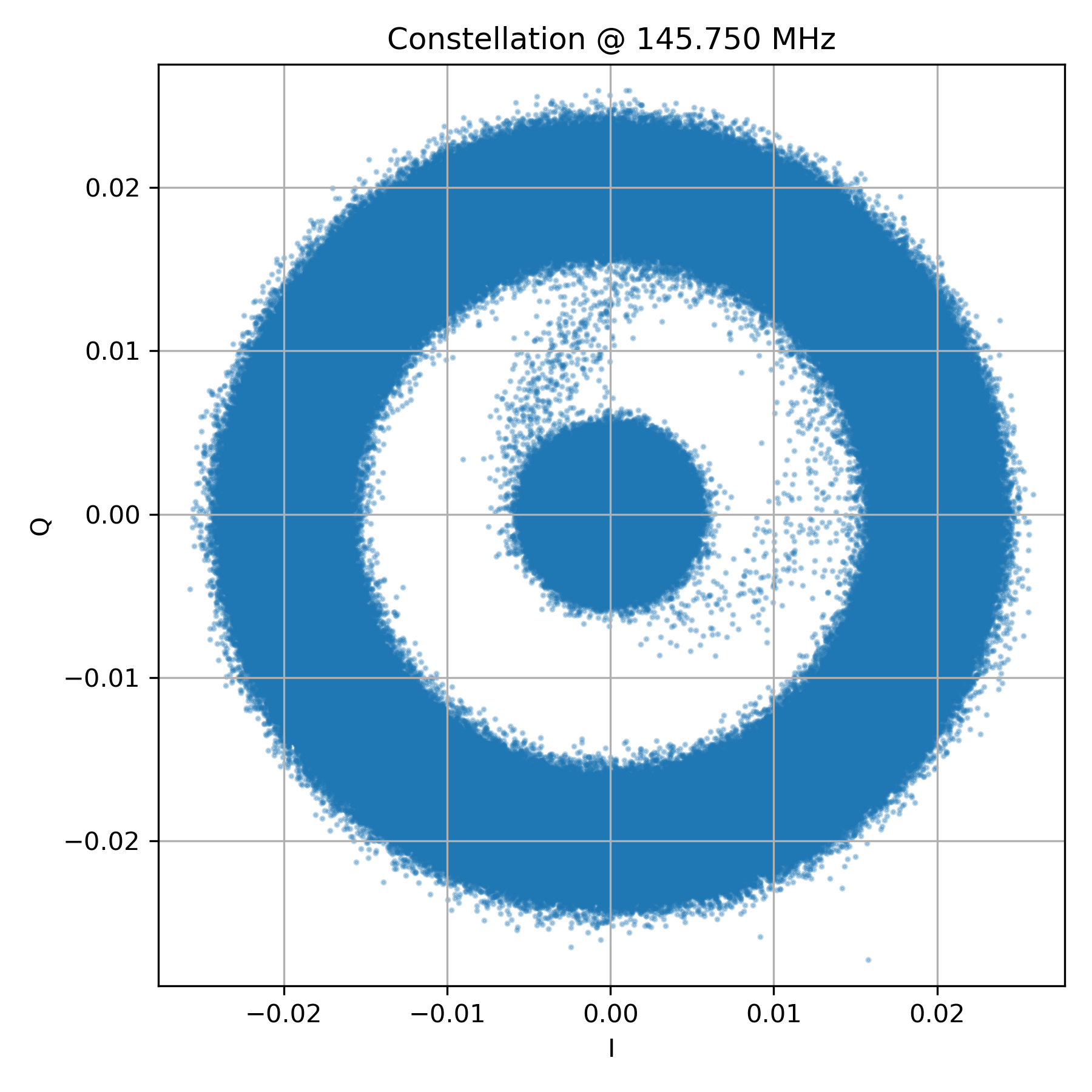
When all IQ samples from the capture are plotted together, the result is less tidy than the broadcast FM case. Instead of a single clean circle, we see a dense central cluster with a surrounding ring.
This immediately tells us something important:
- The repeater is not transmitting continuously
- Large portions of the capture contain only noise
- The central cloud corresponds to periods when the repeater is idle.
With no strong carrier present, the IQ samples collapse toward the origin and form a roughly circular noise distribution.
The ring corresponds to periods when the repeater is active and transmitting FM.
Dynamic IQ: silence, key-up, speech
Animated IQ (GIF, no audio)
# GIF-only animation derived from full animation script
ani.save("dynamic_iq.gif", dpi=80)
Animating the IQ samples reveals the structure much more clearly.
The sequence is easy to follow:
- Silence: a tight, noisy cloud near the origin
- Key-up: a sudden appearance of a rotating ring
- Speech: continuous rotation with changing speed
- Carrier drop: collapse back into noise
This animation reinforces an important idea:
The appearance or disappearance of a carrier is immediately visible in IQ space.
No demodulation is required to see when the repeater is active.
Magnitude vs time: carrier presence
Plot magnitude vs time
mag = np.abs(iq_seg)
plt.plot(t, mag)
plt.xlabel("Time (s)")
plt.ylabel("|IQ|")
plt.show()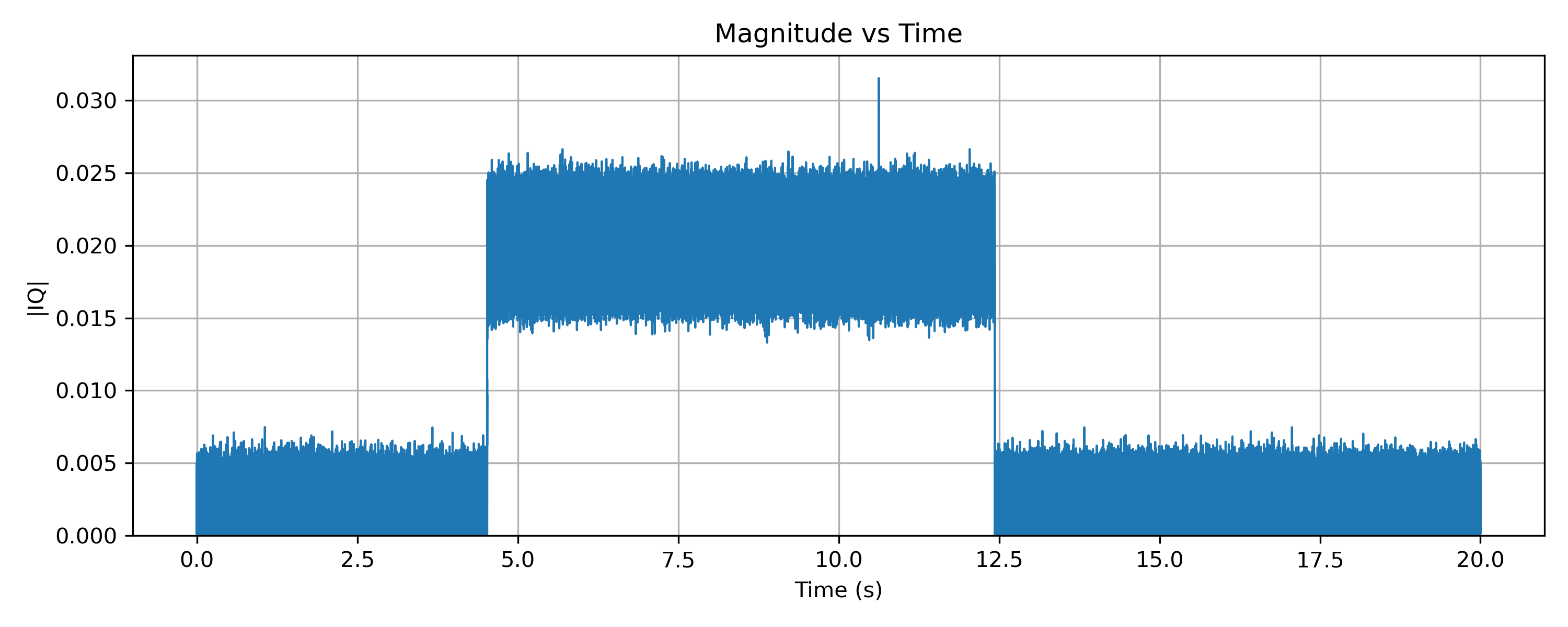
Plotting magnitude against time shows clear steps corresponding to the repeater turning on and off. When the carrier is present, the magnitude rises sharply and remains roughly constant. When the repeater is idle, the magnitude drops back to the noise floor.
As with broadcast FM, the magnitude does not follow the speech itself. This confirms that amplitude is not being used to carry information, even though amplitude changes are useful for detecting transmission boundaries.
Phase and instantaneous frequency
Unwrapped Phase
Unwrapped phase and instantaneous frequency
phase = np.angle(iq_seg)
phase_unwrapped = np.unwrap(phase)

inst_freq = np.diff(phase_unwrapped) * fs / (2*np.pi)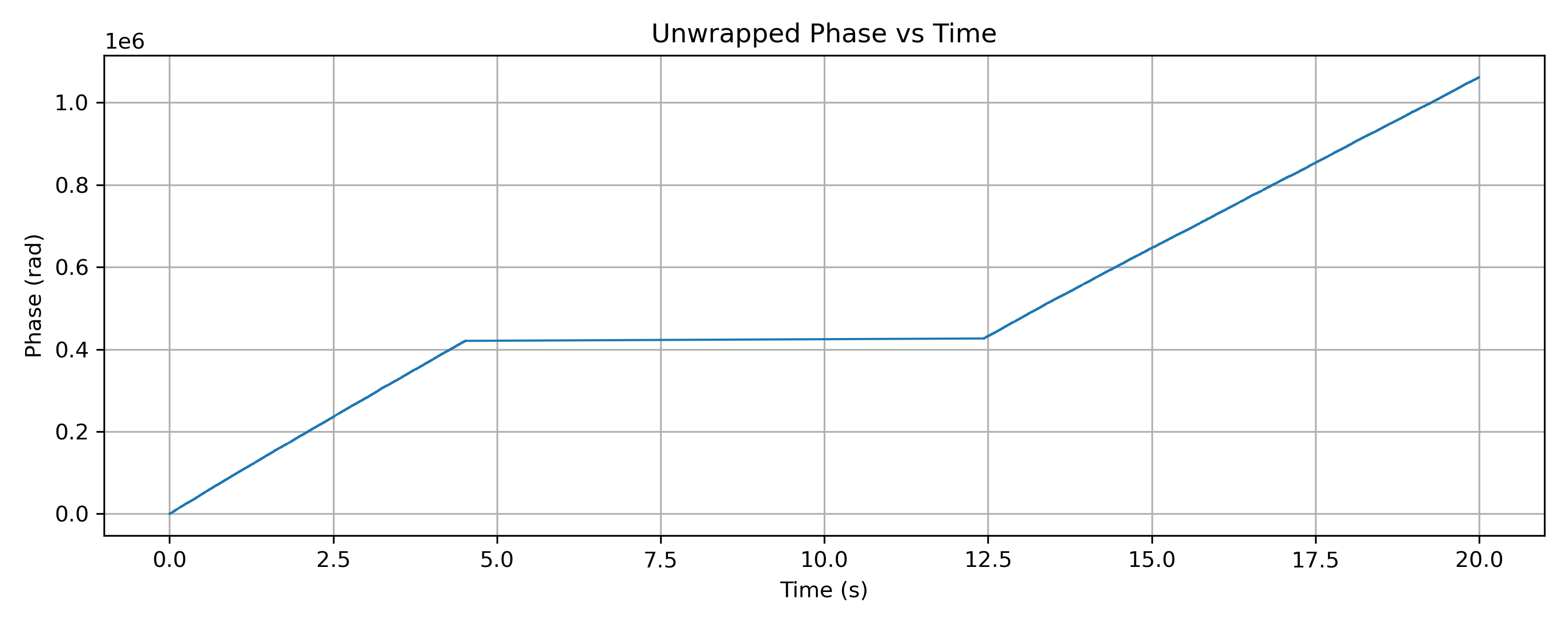
When the repeater is idle, the unwrapped phase shows a roughly diagonal trend rather than a flat line. This arises from the combination of the receiver’s residual frequency offset and the wideband noise present in the capture. In the absence of a coherent carrier, the phase drifts unpredictably and does not reflect any transmitted information.
When the repeater transmits, the phase behaviour changes abruptly. The strong carrier dominates the phase evolution, suppressing the noise-driven drift and producing a more coherent, structured trace.
Rather than revealing the audio modulation directly, the unwrapped phase plot is most useful as a detector of signal presence. It clearly distinguishes periods dominated by noise from periods dominated by a real carrier.
Instantaneous frequency: speech appears
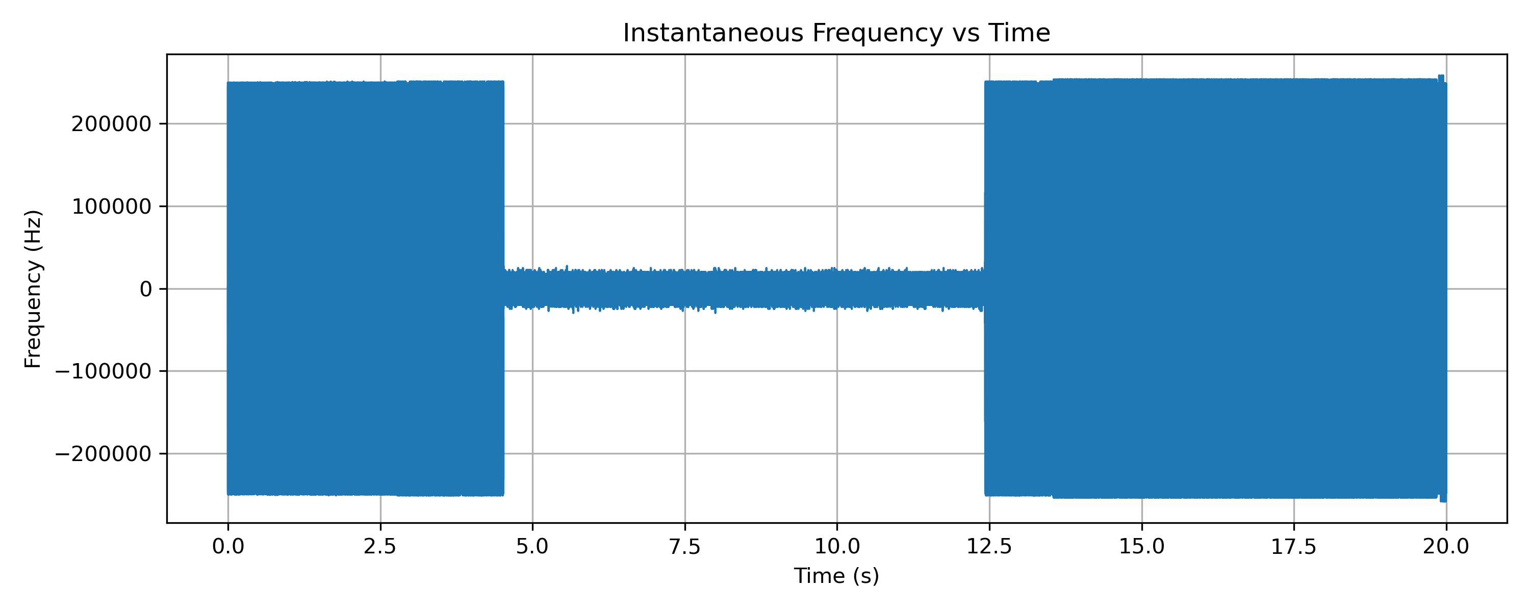
Plotting instantaneous frequency over the full capture highlights the contrast between silence and transmission. During idle periods, the instantaneous frequency spans a very wide range (i.e. ±250 kHz in this 500 kHz capture). These large excursions are not real frequency deviation but arise from differentiating the phase of wideband noise, where instantaneous frequency is essentially meaningless.
When the repeater transmits, the instantaneous frequency collapses into a much narrower band. In this regime, the phase evolves smoothly, and frequency deviation becomes meaningful. The spoken time announcement is visible as structured deviations around the centre frequency, though in practice these deviations are small compared to the noise excursions in idle periods.
Compared to broadcast FM:
- The deviation is narrower
- The audio bandwidth is smaller
- Transitions between silence and speech are more abrupt
This illustrates the operational nature of narrowband FM used on repeaters. In wideband captures, noise dominates the phase and instantaneous frequency outside active transmissions, making the true signal pattern barely readable without filtering or decimation.
The IQ capture shown here spans 500 kHz, integrating noise over a bandwidth far wider than the narrowband FM signal itself. When instantaneous frequency is computed directly on this wideband noise, large and meaningless frequency excursions result.
Real FM receivers apply channel filtering, limiting, and often decimation before demodulation. These steps suppress out-of-band noise, stabilise the phase, and ensure that frequency deviation reflects only the transmitted audio. The unfiltered plots here are shown deliberately, to make the underlying behaviour visible.
Demodulated audio
FM demodulation using active IQ only
active_mask = mag > squelch_thresh
iq_active = iq_seg[active_mask]

phase_active = np.unwrap(np.angle(iq_active))
inst_freq_active = np.diff(phase_active) * fs / (2*np.pi)

audio = filtfilt(b, a, inst_freq_active)
audio /= np.max(np.abs(audio))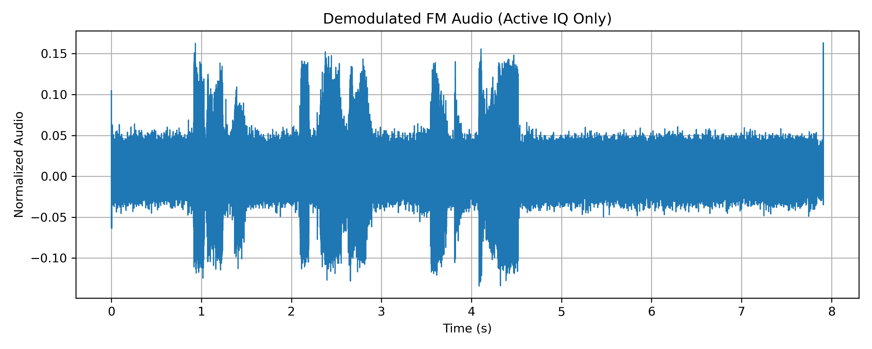
Demodulating the signal using only periods where the carrier is present improves the ability to recover the underlying audio. In practice, receivers interleave filtering and decimation in several stages, progressively reducing bandwidth and sample rate until the signal of interest is isolated and stable enough to demodulate.
The recovered audio appears weaker than the large excursions seen during noise-only periods. This is expected for narrowband FM captured over a wide bandwidth: noise produces large, unstructured phase changes, while speech introduces relatively small frequency deviations.
As before, the demodulated audio is included only as a reference. All of the essential behaviour; carrier presence, silence, speech and transitions; has already been visible in the IQ-derived plots.
Audio-synchronised IQ animation
Synchronising the IQ animation with the demodulated audio makes the relationship between speech and frequency deviation intuitive. As the announcement plays, the rotation rate varies in step with the spoken words; when the audio stops, the rotation vanishes entirely.
What the repeater example adds
Compared to broadcast FM, the repeater example highlights three additional ideas:
- Carriers can appear and disappear, and IQ shows this immediately
- Noise collapses toward the origin in the absence of a signal
- Real-world signals are intermittent, even when the modulation is unchanged
The underlying FM geometry is the same, but the operating context adds structure that is easy to see in IQ space.
GitHub link to code used to create these plots
For complete reproducible scripts, including capture, plotting, and animation, see the GitHub repository.
Where next
So far, all the signals we’ve looked at have used frequency modulation and contained a clear carrier. In the next post, we’ll switch modulation entirely and look at airband AM, where the carrier remains but the information moves from rotation rate to amplitude, producing a very different picture in IQ space.